Gravitational waves

Introduction

Gravitational waves (g-waves) are propagating modes of the gravitational field, and an old prediction from general relativity (GR). They were first proposed in 1916 by A. Einstein himself, and have a tensorial and massless nature. Additionally, g-waves can only be produced by energy-momentum distributions with non-vanishing 2nd order time derivative of their quadrupole (or higher) moments.

G-waves in GR are analog of the electromagnetic waves (e-waves) in Maxwell’s theory of electromagnetism. And, just like light, carry important information about their source. They are irreplaceable when all other channels of radiation (electromagnetic, neutrinos, cosmic rays, etc.) are blocked. For instance, when two black holes coalesce (a BH-BH merger).

This is why g-waves were such a big news a few years back. The first ever detection happened in 2015, when the interferometry observatories LIGO and Virgo simultaneously observed the same BH-BH merger, 1.3 billion light-years away from Earth (LIGO and Virgo Collaborations, 2016). This event, named GW150914, was completely invisible to us otherwise (see Video 1). Thus, its detection represented the birth of a completely new era in astronomy, similar to the first use of the telescope to observe the night sky, done by Galileo Galilei in 1609.

G-waves can also be used in addition to other channels, when they are unblocked. This is known as multichannel or multi-messenger astronomy, and has the potential to revolutionize astrophysics. For example, our understanding of coalescing neutron stars (NS-NS mergers). Such events emit much weaker signals, as they consist of much smaller masses. So, it took longer to detect. But, in 2017, it finally happened. GW170817 was the first (and, so far, the only) NS-NS merger observed via g-waves (LIGO and Virgo Collaborations, 2017).

Approximately 1.7s after GW170817, its electromagnetic counterpart arrived in the form of a short gamma-ray burst, detected by the Fermi and INTEGRAL space telescopes. Finally, approximately 11hs later, the optical part revealed itself as a kilonova, ~140 million light-years away in the lenticular galaxy NGC4994, located at the Hydra constellation. The kilonova was observed by traditional telescopes all around Earth, and lasted a few weeks shinning across all the electromagnetic spectrum — from X-rays to visible light to infrared (check Video 2).

GW150914 and GW170817 are two of the most impactful events in the 21st century physics. The 2016 Special Breakthrough Prize in Fundamental Physics, the 2016 Gruber Prize in Cosmology, the 2017 Breakthrough Of The Year, and the 2017 Nobel Prize in Physics were all dedicated to them.

What are gravitational waves?

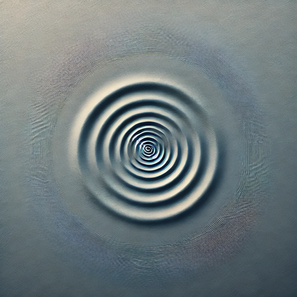
Just like one recognizes small ripples rolling across the surface of a lake as water waves (Figure 1), one could recognize small ripples propagating across the fabric of spacetime as g-waves. This is, of course, quite an idealized scenario, but which helps us understand and easily visualize wave phenomena.

In reality, we know most waves are quite messy and difficult to precisely describe. To illustrate, it is enough to consider a windy day. The surface of the lake might become so choppy it might be hard to distinguish ripples from their surroundings (Figure 2). The lack of clear separation might force you to point to the whole lake as a single wavy mess. And to describe it mathematically, in a nice closed form, might be extremely hard, if not impossible.

The same can happen to spacetime, e.g., in the vicinity of a BH-BH merger. In fact, GW150914 produced so much energy in the form of g-waves, one would have to imagine a wind turbine so powerful, it would outshine the light production of all the stars in the entire observable universe. This was the level of chaos unleashed. Video 3 illustrate how choppy spacetime got in the vicinity of GW150914. Pay attention to the last 20 milliseconds. This is when the g-wave production peaked, and the power output outshone the observable universe 50 times over!

G-waves can very easily produce these messy environments due to their natural non-linear behavior. They are dynamically described by Einstein’s field equations, which consist of 10 non-linear partial differential equations (nPDEs). In vacuum, they read $\mathrm{Ric} = 0$, and look deceptively simple. However, they imply g-waves are described by the curvature of spacetime, and also that g-waves produce and interact with the curvature of spacetime. This is known as backreaction, and has important net effects: g-waves can refract, reflect, redshift, backscatter, damp, etc., all in vacuum.

For comparison, e-waves are much more well-behaved. Dynamically, they are described by Maxwell’s equations which are linear PDEs. In some sense, they are still curvature, but linearity means that it does not interact with itself. Thus, to be messy, light really needs to interact with matter or with gravity. Only then it can refract, reflect, redshift, backscatter, damp, etc.

In addition to the messiness of g-waves, a particularly energetic one can, in principle, undergo gravitational collapse. If focused on a small enough region, it can produce a black hole which destroys a portion of spacetime (geodesic incompleteness). We can hardly call this g-wave a ripple. A catastrophic megatsunami might be more fitting.

As we can see, real g-wave phenomena can be extremely complex. In fact, when serious astrophysicists want to realistically simulate g-wave production, they have no choice but to numerically solve the full set of nPDEs in a supercomputer. Unfortunately, I am not a serious astrophysicist. The g-wave solutions we’re going to discuss next are analytical: they can be written down in terms of elementary functions like $\sin(x)$, $\cos(x)$, $e^x$, etc. Mathematically, they are very nice. However, we should be very aware that “nice mathematics” just cannot cope with the richness of realistic g-waves. In other words, these analytical solutions don’t really exist in nature — they are too idealized. Nevertheless, they are still useful as they carry qualitative features shared with real g-waves. So, I hope you can find them as interesting and illuminating as I do.

PP-wave spacetimes

Due to how the topic of g-waves is taught in undergrad courses all around the world, there is a misconception even among my colleagues, that we need first to linearize $ \mathrm{Ric} = 0 $, in order to get analytical wavy solutions. In other words, that we need to throw away the non-linearities of gravity, making it more similar to electromagnetism. This is, however, not true.

Plane-fronted waves with parallel propagation (pp-waves, for short) is a whole class of exact solutions of Einstein’s equations in vacuum, which describes fully non-linear g-waves. Admittedly, a generic solution in this class is not as immediate to intuitively understand and visualize. But, again, what’s really important is that no unnecessary sacrifices are made. These solutions carry all the non-linear behavior we expect from relativistic gravitational phenomena. Including chaos, caustics, shockwaves, singularity formation, etc.

Consider spacetime to be a Lorentzian 4-manifold $\left(X,g\right)$, where $g(x)$ is known as the metric tensor field. The latter gives us a recipe on how to measure angles and sizes at each event $x \in X$ of spacetime. This is important. Field $g(x)$ is what comes out as solutions to Einstein’s field equations. In other words, it is the fundamental descriptor of gravity in GR.

The family of pp-wave spacetimes consists of all $\left(X, g\right)$ which admits a covariantly constant null vector field $k$. This means $k$ needs to satisfy $g \left(k, k\right) = 0$ and $\nabla k = 0$. The physics savvy reader might be already suspicious that $k$ is the well-known wave vector — and you’re very right! But, at the same time, notice this definition required no physics. It consists of purely mathematical statements belonging to the realm of Lorentzian geometry. In particular, the null vector field condition is always locally guaranteed. What is really restrictive is the covariantly constant condition. This is what makes pp-wave spacetimes mathematically interesting: they contain Petrov type N regions.

Pp-wave spacetimes locally admit the Brinkmann coordinate patch, defined as $\left(u, v, x, y\right) \; ; \; u \in \left(u_0,u_1\right),\; v,x,y \in \left(-\infty, +\infty\right) $, where $k= \partial_{v}$. On it, the metric tensor assumes the form

where $H \left(u, x, y\right)$ is $C^{\infty}$ (smooth) on the $xy$ Euclidean submanifold, $\mathbb{E}^2$, but otherwise arbitrary.

Physics finally kicks in when we demand $g(x)$ to be a solution of $\mathrm{Ric} = 0$. One can show this is equivalent to demand $H$ to be harmonic on $\mathbb{E}^2$. Explicitly, $ \Delta H(u, x, y) = 0$, where $ \Delta \equiv \partial_{x}\partial_{x} + \partial_{y} \partial_{y}$ is the Laplacian differential operator on $\mathbb{E}^2$. No surprise, Einstein’s equations demand $H$ to oscillate (like a wave) in the $xy$ plane. In fact, surfaces of constant $(v_0,u_0)$ can be interpreted as propagating wavefronts!

Clearly, $H$ encodes the particular details of each wavy solution. For instance, if $H = 0$ the metric is just flat Minkowski. If $H$ has compact support, the solution can be interpreted as g-wave packet (pulse). In fact, if $H(u,x,y) = \delta (u) H(x,y)$ we have impulsive g-waves (shockwaves). If $H$ is quadratic in $xy$, the wavefronts have plane geometry: solutions are non-linear plane g-waves. And so on, and so forth.

Post-Minkowskian g-waves

Now that we cleared out some misconceptions, let’s address the more pedagogical approach — the one usually taught in undergrad courses. The end result is way easier to visualize, but to the expense of exactness. They’re only approximations of already idealized solutions.

Let’s first establish the simplest solution to Einstein’s equations in vacuum: the already mentioned Minkowski spacetime. This is the globally flat manifold denoted by $\left(X,\eta\right)$, where

\[\eta \left(x\right) = -dt^2 + dx^2 + dy^2 + dz^2 \;,\]

and $t,x,y,z \in \left(-\infty, +\infty\right)$ is the globally defined Cartezian patch. Because Minkowski is everywhere flat, it is also destitute of any gravitational fields. One could say it is the lowest energy, most boring solution of $\mathrm{Ric} = 0$. Thus, it is the perfect background to study how ripples propagate.

Second, we want to describe a scenario similar to Figure 1, where there is a clear separation between ripples and their surrounding background. In other words, a solution equivalent to “$\eta$ plus ripples”. Mathematically, we propose $g’ = f^{\ast} g \; ; \; g’ \equiv \eta + h$, where $f: \left(X,g’\right) \rightarrow \left(X,g\right)$ is a diffeomorphism.

The equation $g’ = f^{\ast} g$ means $g$ is equivalent to $g’$. This is because Einstein’s field equations are covariant under transformation $f$. Saying it differently, $g$ and $g’$ represent the same physical solution: Minkowski with ripples. To be clear, $h(x)$ is a symmetric rank-2 tensor field representing these ripples. Mathematically, if $g$ is a solution, then $g’$ is a solution as well, which means $\mathrm{Ric} \left(g’, \partial g’, \partial^{2} g’\right) = 0$. Moreover, we also know $\eta$ is yet another solution — in fact, the globally constant most boring one, $\partial \eta = \partial^2 \eta = 0$ — which brings the final result to

\[\mathrm{Ric} \left(\eta, h, \partial h, \partial^2 h\right) = 0 \;. \label{eq:einstein-eq-for-h} \tag{1}\]

We clearly achieved separation since Einstein’s equations now became differential only for $h$. One could say we’re now dealing with a traditional $h$ field theory over a fixed Minkowski background. This is known as the post-Minkowskian regime of GR. The only “problem” is that \eqref{eq:einstein-eq-for-h} is still nonlinear, which means complicated dynamics and potentially messy solutions just like before. Our next step is to find a way to simplify this by discarding all the non-linearities, a.k.a., let’s make gravity similar to the electromagnetism.

Perturbation theory

The messiness brought by non-linearities can manifest in the real world as caustics, shockwaves, phase transitions, turbulence, singularities, etc. Thus, it is nothing but reasonable to expect $h$ to be, at the very most, a $C^{\infty}$ field. In fact, \eqref{eq:einstein-eq-for-h} only demands it to be $C^2$ (twice differentiable). Figure 2, again, represents quite an extreme case — but not at all uncommon — in which smoothness is definitely absent, and $C^0$ (continuity) is questionable.

One way to control these complexities is to demand $h$ to be $C^{\omega}$ (analytic¹). This is quite a restrictive assumption, which is only satisfied by a very small fraction of all possible solutions to \eqref{eq:einstein-eq-for-h}. Analyticity forbids caustics, singularities, phase transitions, etc., but also $h$ to be compactly supported on $X$. If a $C^{\omega}$ solution has compact support, then it is necessarily trivial (everywhere vanishing). This is because every $C^{\omega}$ solution is globally determined by its behavior in a local neighborhood of its domain — which is also a non-causal feature. If it vanishes somewhere, it has to vanish everywhere. Thus, every non-trivial $C^{\omega}$ solution is necessarily eternal and omnipresent (globally type N), and incapable of describing g-wave generation by localized sources.

At times, analyticity might be a physical sacrifice worth paying for. Pedagogically, $C^\omega$ solutions are easier to understand and visualize. They are computationally simple to obtain. And, physically, some of them still share qualitative features with their more physical non-analytic counterparts. If $h$ is assumed $C^{\omega}$ on $X$, then it has an exact representation in terms of a Taylor series,

\[h (x) = \sum_{n=0}^{\infty} \frac{1}{n!}\nabla_{\dot{\gamma}(0)}^{(n)} h \mid_{\gamma (0)} \;, \label{eq:taylor-series} \tag{2}\]

where $\gamma: [0,1] \rightarrow X$ is a smooth curve connecting $\gamma (0) \equiv x_0 $ to $\gamma (1) \equiv x$. Again, the right-hand side of \eqref{eq:taylor-series} is a convergent power series locally defined in the neighborhood of $x_0$, but which determines $h(x)$ over the entire $X$.

A less restrictive way to control the non-linearities is to assume the domain of $h$ admits an asymptotic scale, denoted by the set of fields $ \{ h^{(n)}(x) \} $. In this case, $h$ just needs to be $C^{0}$, and we technically keep most of its non-analytic behavior. However, there is a mathematical price to be paid. Equation \eqref{eq:taylor-series} erodes into an equivalence to an asymptotic expansion,

\[h(x) \sim \sum_{n=0}^{\infty} h^{(n)}\;. \label{eq:asymptotic-series} \tag{3}\]

The right-hand side of \eqref{eq:asymptotic-series} is what mathematicians call a formal series. Contrasting \eqref{eq:taylor-series}, this infinite sum has no obligation to converge to a finite quantity, much less one equal to $h(x)$. Fortunately, \eqref{eq:asymptotic-series} is not pure mathematical wizardry, and we can give a rigorous meaning to $\sim$. For any finite truncation, the reminder

\[\mathcal{R}_N (x) \equiv h - \sum_{n=0}^N h^{(n)}\]

has to be strictly smaller than the leading order as $x$ approaches the future null infinity $\mathcal{I}^+$ of $\left(X,\eta\right)$. With this restriction, it is possible to define an equivalence class in which \eqref{eq:asymptotic-series} rigorously holds.

Physicists like to call either of these techniques perturbation theory. The goal is to find a truncation of either \eqref{eq:taylor-series} or \eqref{eq:asymptotic-series}, depending on your assumptions, which approximates “well enough” the exact solution you’re trying to study. The higher the truncation order you need, the bigger is the piece you have to evaluate. The bigger the piece, the better the approximation is. However, these methods have very quickly diminishing returns.

The leading order is always the 1st, which is also the linear limit. Beyond leading order truncations represent non-linear effects being carefully introduced as ever smaller corrections. At high orders, we pay a very large computational price for a very tiny improvement. Thus, most research is done at the leading order. Nonetheless, there are occasions one would consider 2nd order truncations. After all, they give the first glimpse of how non-linear effects come into play.

Linear g-waves

The $N=0$ truncation is just a constant. Minkowski plus a constant is diffeomorphically Minkowski again. Thus, the $0$-th order truncation is too low to result in anything interesting. Substituting \eqref{eq:asymptotic-series}, truncated at $N=0$, into \eqref{eq:einstein-eq-for-h}, just trivially results in the statement that Minkowski is globally flat — again, something we already knew.

Now, as stated before, the 1st order is the leading order, which is also the linear limit. Substituting \eqref{eq:asymptotic-series}, truncated at $N=1$, into \eqref{eq:einstein-eq-for-h}, results in

\[\Box h^{(1)} = 0 \;, \label{eq:linear-g-wave} \tag{4}\]

where $\Box \equiv \partial \cdot \partial$ is the d’Alembertian differential operator on Minkowski spacetime, and the gauge fixing condition, $\partial \cdot \bar{h}^{(1)} = 0$, was used². Now, this is something new. In fact, this is what Einstein found in 1916! Apart from the fact $h^{(1)}$ is tensorial, \eqref{eq:linear-g-wave} is the same mathematical equation which governs the dynamical behavior of e-waves in vacuum. In other words, at leading order in the post-Minkowskian approximation, Einstein’s field equations forces $h$ to behave as traditional linear waves.

For an arbitrary truncation, we generally end up with

\[\Box h^{(N)} = f^{(N)} \;,\]

where $f^{(N)}$ is a function depending non-linearly on $h^{(N-1)}$ and its derivatives. So, the beyond leading order behavior is clear. The $N$-th order non-linearities, contained in $f^{(N)}$, are constructed out of the $(N-1)$-th order solutions, and behave as sources for $h^{(N)}$. Again, we see that non-linearities introduce self-interactions. In particular, higher order g-waves are generated by lower order g-waves: gravity generating gravity.

We have to mention that truncations will inevitably break the diffeomorphism symmetry (covariance) of Einstein’s equations. The good news is that the breakage is only partial. This detail is actually quite important for the physics of g-waves. At leading order, an Abelian gauge symmetry remains, given by the field transformation

\[h^{(1)} \mapsto {h'}^{(1)} = h^{(1)} + L_{\xi} \eta \;, \tag{5}\label{eq:gauge-symmetry}\]

where $L_{\xi}$ is the Lie derivative along the smooth vector field $\xi$. Condition $ \partial \cdot \bar{h}^{(1)} = 0 $, used to gauge fix this symmetry, simplifed the dynamical equations in \eqref{eq:linear-g-wave}. However, most gauge fixings are flawed, and this one is no exception. So much so, \eqref{eq:gauge-symmetry} is a symmetry of $ \partial \cdot \bar{h}^{(1)} = 0$ itself, if $\Box \xi = 0$. In summary, there are still gauge redundancies in \eqref{eq:linear-g-wave} which need to be addressed before we can speak of the actual physical degrees of freedom (DoF) g-waves represent.

The linear plane wave

Ironically, the most straightforward solution to \eqref{eq:linear-g-wave} is an analytic solution known as the monochromatic linear plane wave,

\[h^{(1)} = \mathrm{Re} \left( A e^{i k \cdot \mathbb{x}}\right) \;,\]

where $\mathrm{Re} (z) \equiv \left(z+\bar{z}\right)/2$ is the real part of $z \in \mathbb{C}$; $A$ is a real symmetric rank-2 tensor field known as the polarization tensor ; $k$ is the wave vector; and, $\mathbb{x} \equiv x^{\mu}\partial_{\mu}$ is the Euler vector field. There is nothing too complicated here, in fact, the piece $\mathrm{Re} (e^{ik \cdot \mathbb{x}}) = \cos (k \cdot \mathbb{x})$ just gives how $h^{(1)}$ oscillates, and $A$ gives the directions in which these oscillations happen.

Monochromatic (single color) implies $h^{(1)}$ has a well-defined constant frequency. Consequentially, $k$ is a globally constant field, immediately satisfying $\nabla k = 0$. Moreover, \eqref{eq:linear-g-wave} imposes $\eta \left(k,k\right) h^{(1)} = 0$ on this solution. If $h^{(1)}$ is to be non-trivial, then necessarily $\eta(k,k)=0$. Together, these conditions indeed imply massless modes travelling along null geodesics to which $k$ is tangent to. In other words, GR predicts g-waves travelling exactly at the speed of light. They also imply that the “Minkowski plus ripples” spacetime, at leading order $\left(X, \eta + h^{(1)}\right)$, is a legit member of the bigger class of pp-wave spacetimes.

The equation $k \cdot \left( \mathbb{x} - \mathbb{x}_0 \right) = 0$ defines an infinite family of parallel planes — each plane labelled by a particular value of the vector field $\mathbb{x}_0$. This equation also states that $k$ is normal to these planes: the planes can be interpreted as wavefronts. This is where the name plane wave comes from. Additionally, the gauge fixing condition imposes $h^{(1)}(k) = 0$. Consequentially, all oscillatory behavior is confined to the wavefronts, i.e., $A$ doesn’t have a projection on the $k$-direction. This property cements g-waves as transverse waves.

As promised, $C^{\omega}$ solutions are way easier to understand and work with, but they’re also quite artificial. We can clearly see that linear plane waves are eternal (wavefronts extend indefinitely to the past and to the future) and have an unrealistically high degree of symmetry (wavefronts are planes). Nonetheless, when interacting with matter they can still reflect, refract, diffract, etc., as any other wave does. So, a lot of real physics can be done with them.

Polarization modes

A peculiar feature of transverse waves is known as polarization. It describes changes in the oscillation direction of $h^{(1)}$ as each wavefront arrives. Mathematically, polarization is captured by $A$. Physically, it represents the most elementary DoF of a g-wave: all the independent variables that satisfy the dynamical equations, but also survive all the gauge fixing constraints.

We introduced the g-wave ripple as the symmetric rank-2 tensor. In four spacetime dimensions, this means 10 field variables. However, at leading order, we also introduced the gauge fixing condition, $\partial \cdot h^{(1)} = 0$. This implicitly suggests that at least 4 of these variables are dependent, i.e., they’re gauge redundancies (non-physical artifacts of a gauge symmetry).

In preparation for this section, we did mention that our gauge fixing was not perfect. In other words, there are still gauge artifacts among these 6 field variables we’re left with. To get rid of them all, we need to fully fix symmetry \eqref{eq:gauge-symmetry}. This is done by enhancing our previous gauge fixing. The so-called transverse traceless synchronous (TTS) gauge is defined by

\[\partial \cdot h^{(1)} = 0 \;, \tag{transverse}\] \[\tr \left(h^{(1)}\right) = 0 \;, \tag{traceless}\] \[h^{(1)} \left(\partial_{t}\right) = 0 \;, \tag{synchronous}\]

and represents a total of 8 independent constraints. In this gauge, it is very clear that $h^{(1)}$ have only 10-8=2 independent field variable, i.e., 2 physical DoF. These are known as the 2 polarization modes allowed for g-waves.

The TTS gauge constraints concomitantly imply that the gauge symmetries acting upon g-waves are such that scalar, vectorial and traceful tensorial modes are all pure gauge, i.e., they don’t really propagate. Thus, g-waves have no other option but to be fundamentally tensorial traceless. Tensorial means it acts “volumetrically”, like stress in a material body. Traceless means it preserves angles, but not necessarily sizes (as we will see). This is also why they’re only excited by higher multipole moments of matter. The monopole and dipole couple to these pure gauge modes, and thus aren’t able to produce gravitational radiation.

As we just mentioned, being traceless and tensorial leaves g-waves with only two independent ways of being different. These are the so-called $+$ and $\times$ polarization modes. To visualize these modes, consider $h^{(1)}$ propagating in the $\partial_z $-direction, namely, $k= \omega \partial_{t} + k_z \partial_{z}$. To satisfy $\eqref{eq:linear-g-wave}$, the null condition $\eta \left(k,k\right)=0$ needs to be respected. This means $\omega = k_z$. Now, to satisfy the TTS gauge, $A$ can only be given by 2 free parameters. In a very convenient frame, its matrix notation reads

\[\left[A \left(\partial_{\mu}, \partial_{\nu}\right)\right] = \begin{bmatrix} 0 & 0 & 0 & 0 \\ 0 & A_{+} & A_{\times} & 0 \\ 0 & A_{\times} & -A_{+} & 0 \\ 0 & 0 & 0 & 0 \end{bmatrix} \;.\]

Quite clearly we can decompose this in a linear combination of the $+$ and $\times$ modes,

\[h^{(1)} = h^{(1)}_{+} + h^{(1)}_{\times} \;,\]

where

\[\left[ h^{(1)}_{+} \left(\partial_{\mu}, \partial_{\nu}\right)\right] \equiv A_{+}\begin{bmatrix} 0 & 0 & 0 & 0 \\ 0 & 1 & 0 & 0 \\ 0 & 0 & -1 & 0 \\ 0 & 0 & 0 & 0 \end{bmatrix} \mathrm{Re} \left[ e^{i \omega ( t-z )} \right] \;,\]

and

\[\left[ h^{(1)}_{\times} \left(\partial_{\mu}, \partial_{\nu}\right)\right] \equiv A_{\times}\begin{bmatrix} 0 & 0 & 0 & 0 \\ 0 & 0 & 1 & 0 \\ 0 & 1 & 0 & 0 \\ 0 & 0 & 0 & 0 \end{bmatrix} \mathrm{Re} \left[ e^{i \omega ( t-z )} \right] \;.\]

Notice this frame is quite special. In it, $h_{+}^{(1)}$ and $h_{\times}^{(1)}$ differ only by a similarity transformation,

\[h_{\times}^{(1)} = \frac{A_{\times}}{A_{+}} \mathcal{R}^T \left(\frac{\pi}{4}\right) h_{+}^{(1)} \mathcal{R} \left(\frac{\pi}{4}\right) \;, \tag{6} \label{eq:similarity-transform}\]

where $\mathcal{R}(\theta)$ is the rotation operator, along the $z$ axis, by an angle $\theta$. In simpler terms, if you look at a g-wave from a particular angle, its modes look indistinguishable from each other! However, we emphasize that this is not a frame-independent reality.

Let’s physically interpret $h_{+}^{(1)}$. If $A_{+}\mathrm{Re} \left[e^{i \omega (t-z)}\right] >0$, its polarization tensor implies that, as each wavefront passes, the $xx$ component of the “Minkowski plus ripple” metric scales up, while the $yy$ component scales down. If $A_{+}\left[e^{i \omega (t-z)}\right] < 0$, then the opposite happens.

We did say quite a while ago that metrics are of fundamental importance as they give us a recipe on how to measure sizes and angles in a space. The angles here are left untouched because, as we’ve established, g-waves are traceless. Thus, the passage of $h_{+}^{(1)}$ fundamentally alters our notion of sizes in the $xx$ and $yy$ directions. Meanwhile, the passage of $h_{\times}^{(1)}$ does exactly the same, but rotated $\pi/4$ radian (45°) in the $xy$ plane (see Animation 1).

A monochromatic plane g-wave is, in general, a linear combination of $h_{+}^{(1)}$ and $h_{\times}^{(1)}$ (see Animation 2). And, to obtain the most general linear g-wave, we have to sum over all possible monochromatic linear g-waves. Namely,

\[h^{(1)} = \mathcal{F} \left[ h_{+}^{(1)} + h_{\times}^{(1)}\right] \;,\]

where $\mathcal{F}$ is a Fourier transform from the space of frequencies. Keep in mind though, this only holds true at leading order.

Detectors’ designs

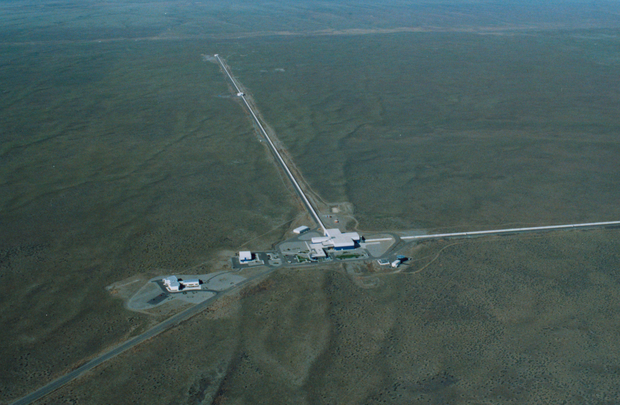
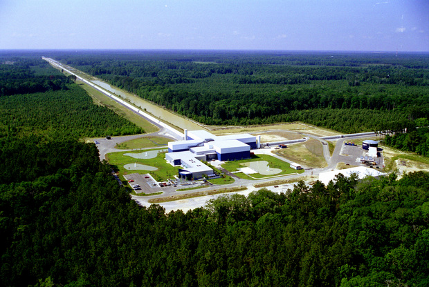
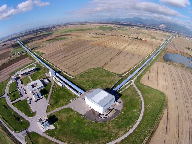
Finally, to finish our discussion, we point out why g-waves observatories like LIGO and Virgo are made of 2 long arms separated by the most perfect 90° angle, check Photos 1–3.

To understand this unique design, we have to understand how we perceive an incoming g-wave. First, it’s very rare for a g-wave to have exactly the same amplitudes for both $+$ and $\times$ modes. It is too coincidental, especially considering the chaotic environment they originate from. Additionally, the angle at which a g-wave hit us plays a very important role.

Consider a compact binary system as source, and that its plane of orbit is parallel to the detector’s plane, a.k.a., the g-waves would hit us head on. Looking at Animation 1, it is very clear that this detectors’ design maximizes the stretching/compressing effect on each of its arms. The 90° separation was carefully chosen to cap the detectors’ sensitivity. Unfortunately, this is not a free meal. In this kind of arrivals, this design also preserves axial symmetry. As a direct consequence of similarity transformation \eqref{eq:similarity-transform}, this means it is impossible to distinguish between $+$ and $\times$ polarization modes. In summary, we have maximum sensitivity for head on arrivals at the cost of perceiving the g-waves as almost purely polarized (which qualitatively is Animation 1).

Now, if the binary’s plane of orbit and the detectors’ plane are not parallel, then the g-waves would hit us at an angle. Axial symmetry would then be broken, and we would be able to quantify the individual contribution of each polarization mode. Of course, different angles give us different ratios $A_{+}/A_{\times}$. Our sensibility to each mode reaches a maximum when the planes are perpendicular, a.k.a., the g-waves hit us edge on (which qualitatively is Animation 2). However, this is also when the stretching/compressing effect on the arms are minimum. In other words, we’re best at distinguish the polarization modes when we’re the worst at detecting the overall wave.

It is clear that this design is biased towards purely polarized head on arrivals. The initial priority of the LIGO and Virgo collaborations was to ensure the first ever detection of a g-wave, not really to study its detailed nature. This strategy really paid off, and also highlights the need of multiple detectors, at different places and orientations, scattered around the globe.

Something similar can be said about the length of each arm. The stretching/compressing in Animations 1–2 are highly exaggerated for visualization purposes. In practice, these arrive at Earth as extremely tiny perturbations (smaller than the typical width of atomic nuclei). We would need an extremely long pair of arms to have any significant absolute displacement. Currently, LIGO and Virgo operate at the very technological limit of Earth-based detectors, each arm being 3 and 4 kilometers long, respectively.

To remove the shortcomings of Earth-based detectors, the next generation is going to be space-based. LISA is designed to have arms 2.5 million km long — you read that right, 2.5 million kilometer each arm! Also, you can immediately see (Figures 3–4) they’re configured quite differently: they close in an equilateral triangular shape.

Lisa is not biased towards head-on arrivals. As it trails Earth in its orbit around the Sun, the triangle slowly changes orientation. In a year, Lisa sweeps the entire celestial sphere, averaging out any arrival bias. Additionally, due to the $\pi/3$ rad (60°) separation between the arms, LISA breaks the similarity transformation which degenerates the $+$ and $\times$ modes. In summary, LISA is designed for a very detailed study of g-waves. It has full sky coverage, and it is always able to pinpoint the precise composition of a g-wave in terms of its polarization modes.

In general, next-gen detectors represent an increase between $10^2$ to $10^3$ times our current sensibility, allowing us to observe the gravitational wave background (GWB). This is made of low-frequency g-waves which permeates the entire universe, analogous to the electromagnetic cosmic microwave background (CMB). The GWB has many possible origins, from primordial cosmological phase transitions such as the inflationary re-heating, and the electroweak phase transition, to cosmic strings. Less speculative contributions are expected from supermassive BH-BH mergers, stellar mass BH-BH mergers, supernovae, etc. All very exciting stuff.

References